%load_ext autoreload
%autoreload 2
from logistic import LogisticRegression, GradientDescentOptimizer
The autoreload extension is already loaded. To reload it, use:
%reload_ext autoreload%load_ext autoreload
%autoreload 2
from logistic import LogisticRegression, GradientDescentOptimizerThe autoreload extension is already loaded. To reload it, use:
%reload_ext autoreloadMy implementation of the logistic regression algorithm (logistic.py) can be found here.
In this blog post we will explore the implementation of logistic regression and focus on optimizing the binary cross-entropy loss through gradient descent with momentum. We will validate and explore the model we implemented through several experiments on synthetic datasets. We will observe both vanilla gradient descent and momentum-enhanced gradient descent and hwo the latter can improve the speed of our models. We will also examine the challenges of overfitting by working with high-dimensional data sets. Finally, we will apply our logistic regression model to predict FIFA World Cup match outcomes using real-world statistics and highlight the challenges and benefits therein. Through these experiments, we illustrate the advantages and trade-offs between convergence efficiency and model generalizability, and offer some thoughts on practical classification tasks and possible future work.
The logistic regression model I implemented minimizes the binary cross-entropy loss to classify data. During training, we use momentum to help the model move more quickly in the right direction by combining the current gradient with a fraction of the previous update as we try search the loss-space for a minimum. The momentum should help reduce oscillations and speed up convergence! Lets see how it works!
We will start with vanilla gradient descent. We will be working with two-dimensional data (x1, x2) and setting our \(\beta\) value to zero to nullify the momentum term.
The code below provides functions to generate and plot data for a classification problem that we can address using our model. To test our vanilla model, lets generate some linearly separable data!
import torch
import numpy as np
import matplotlib.pyplot as plt
plt.style.use('seaborn-v0_8-whitegrid')

# torch.manual_seed(67)

def classification_data(n_points = 300, noise = 0.2, p_dims = 2):

    y = torch.arange(n_points) >= int(n_points/2)
    y = 1.0*y
    X = y[:, None] + torch.normal(0.0, noise, size = (n_points,p_dims))
    X = torch.cat((X, torch.ones((X.shape[0], 1))), 1)

    return X, y

def plot_lr_data(X, y, ax):
    assert X.shape[1] == 3, "This function only works for data created with p_dims == 2"
    targets = [0, 1]
    markers = ["o" , ","]
    for i in range(2):
        ix = y == targets[i]
        ax.scatter(X[ix,0], X[ix,1], s = 20,  c = 2*y[ix]-1, facecolors = "none", edgecolors = "darkgrey", cmap = "PRGn", vmin = -2, vmax = 2, alpha = 0.5, marker = markers[i])
    ax.set(xlabel = r"$x_1$", ylabel = r"$x_2$")

fig, ax = plt.subplots(1, 1, figsize = (4, 4))
X, y = classification_data(noise = 0.2, p_dims = 2)
plot_lr_data(X, y, ax)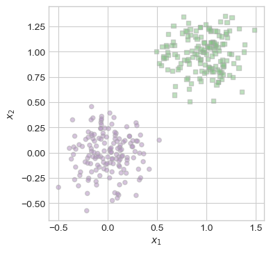
LR = LogisticRegression()
opt = GradientDescentOptimizer(LR)

loss_vec_vanilla = []
max_iter = 1000

for _ in range(max_iter):
    loss = LR.loss(X, y)
    loss_vec_vanilla.append(loss)

    opt.step(X, y, alpha=0.45, beta=0)

losstensor(0.0140)Thats great! Looks like we were able to separate the data by achieving a minimal loss! Lets take a look at the line that separates our points.
def draw_line(w, x_min, x_max, ax, **kwargs):
    w_ = w.flatten()
    x = torch.linspace(x_min, x_max, 101)
    y = -(w_[0]*x + w_[2])/w_[1]
    l = ax.plot(x, y, **kwargs)

fig, ax = plt.subplots(1, 1, figsize = (4, 4))
plot_lr_data(X, y, ax)
draw_line(LR.w, x_min = -0.5, x_max = 1.5, ax = ax, color = "slategrey")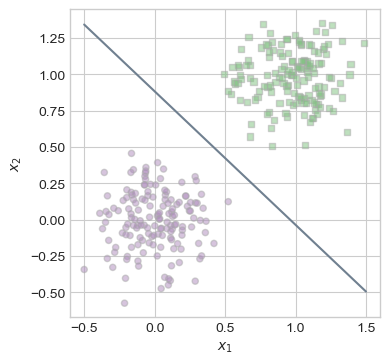
As seen above, our line very handily separates the two classes of points. Lets take a look at how our loss evolved over time by plotting our loss at each step.
plt.plot(loss_vec_vanilla, color = "purple", lw=2)
# plt.scatter(torch.arange(len(loss_vec)), loss_vec, color = "purple")
labs = plt.gca().set(xlabel = "Logistic Regression Iteration", ylabel = "loss")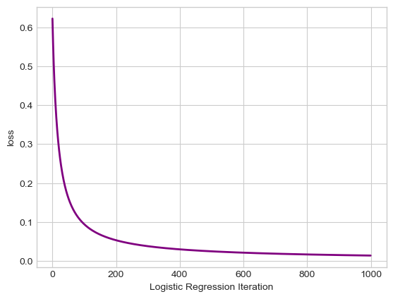
It is interesting to note that our Logistic Regression is not jumping around as we observed with the Perceptron algorithm in the previous blog post. On the contrary, using gradient descent on a convex loss function, we are slowly advancing towards the minimum of the function.
Now lets look at how momentum can help us! We will use the same dataset, however, this time we will instantiate a model with a \(\beta=0.9\).
LR = LogisticRegression()
opt = GradientDescentOptimizer(LR)

loss_vec_momentum = []

for _ in range(max_iter):
    loss = LR.loss(X, y)
    loss_vec_momentum.append(loss)

    opt.step(X, y, alpha=0.45, beta=0.9)

losstensor(0.0020)Lets see how these processes stack up against each other. For the graph we are
num_iter = 500
plt.plot(loss_vec_vanilla[:num_iter], color = "purple", lw=2, label = "vanilla")
plt.plot(loss_vec_momentum[:num_iter], color = "blue", lw=2, label = "momentum")
labs = plt.gca().set(xlabel = "Logistic Regression Iteration", ylabel = "loss", title = f"Momentum vs. Vanilla Gradient Descent (first {num_iter} iterations)")
plt.legend()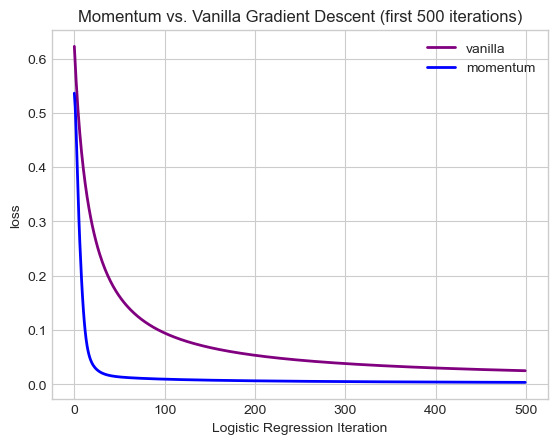
As we can see, including a momentum factor helps the model narrow in on the minimum loss a lot faster! When we use vanilla, we are updating our weight vector only using teh current gradient. However, with momentum we are also considering the direction of the previous update, so we build up momentum when we are going the right direction which helps us find the minimum faster.
Next, we are going to take a look at some issues pertaining to overfitting our model. We are going to generate data where the the number of features is higher than the number of points we have, p_dim > n_points. To illustrate the issues of overfitting, we will generate separate testing and validation data sets, then compare their accuracy.
X_train, y_train = classification_data(noise = 1.2, p_dims = 100, n_points = 50)
X_test, y_test = classification_data(noise = 1.2, p_dims = 100, n_points = 50)
Here is a small helper function to calculate our accuracy.
def acc(model, X, y):
    y_hat = model.predict(X)
    return (y_hat == y).float().mean().item()
Now lets train a model that achieves 100% training accuracy!
LR = LogisticRegression()
opt = GradientDescentOptimizer(LR)

train_loss = []
test_loss = []

for _ in range(50):
    train_loss.append(LR.loss(X_train, y_train))
    test_loss.append(LR.loss(X_test, y_test))

    opt.step(X_train, y_train, alpha=0.5, beta=0.9)

train_acc = acc(LR, X_train, y_train)
print(f"Training Accuracy: {train_acc * 100:.2f}% Training Loss: {LR.loss(X_train, y_train):.4f}")
Training Accuracy: 100.00% Training Loss: 0.0000Voila! This seems amazing! We have 100% accuracy and a very low loss! However, our testing data may not ignite the same happiness within us.
test_acc = acc(LR, X_test, y_test)
print(f"Test Accuracy: {test_acc * 100:.2f}% Test Loss: {LR.loss(X_test, y_test):.4f}")
Test Accuracy: 88.00% Test Loss: 1.1519Youch. This is a lot lower accuracy that we would have liked. In addition, the testing loss is quite high! Lets have a look at how our model performs at each iteration.
plt.plot(train_loss, color = "green", lw=2, label = "Training")
plt.plot(test_loss, color = "orange", lw=2, label = "Testing")
labs = plt.gca().set(xlabel = "Logistic Regression Iteration", ylabel = "loss", title = f"Training vs Testing Loss")
plt.legend()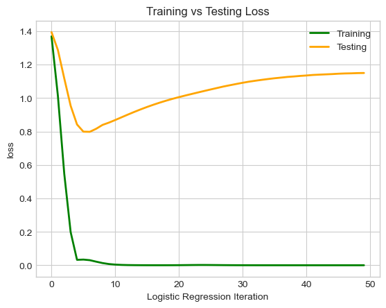
We can see our training loss decrease and converge to zero, however, at a certain point our testing loss that was once decreasing too, begins to increase! The model continues to learn (and thus overfit) the training data, even as it starts to perform worse on generalizing to new data. When we have a higher number of features than we do samples, overfitting can become problematic as it did above.
To illustrate our Logistic Regression model on some empirical data, we are going to use World Cup Match Data and try and predict match winners! The dataset we are using was compiled on Kaggle by Brenda Loznik in 2022 from publicly available FIFA World Cup data. Players were manually classified as either goalkeeper, defender, midfielder, or offensive player. For each team, only the top-performing players were selected. These plater statistics were used to create the power scores for each team. In some cases, data is missing — this indicates that a country did not have enough qualifying players to met the selection criteria. Additionally, the dataset assumes that each season runs from September to the following August.
import pandas as pd
df = pd.read_csv('international_matches.csv')
df.head()| date | home_team | away_team | home_team_continent | away_team_continent | home_team_fifa_rank | away_team_fifa_rank | home_team_total_fifa_points | away_team_total_fifa_points | home_team_score | ... | shoot_out | home_team_result | home_team_goalkeeper_score | away_team_goalkeeper_score | home_team_mean_defense_score | home_team_mean_offense_score | home_team_mean_midfield_score | away_team_mean_defense_score | away_team_mean_offense_score | away_team_mean_midfield_score | |
|---|---|---|---|---|---|---|---|---|---|---|---|---|---|---|---|---|---|---|---|---|---|
| 0 | 1993-08-08 | Bolivia | Uruguay | South America | South America | 59 | 22 | 0 | 0 | 3 | ... | No | Win | NaN | NaN | NaN | NaN | NaN | NaN | NaN | NaN |
| 1 | 1993-08-08 | Brazil | Mexico | South America | North America | 8 | 14 | 0 | 0 | 1 | ... | No | Draw | NaN | NaN | NaN | NaN | NaN | NaN | NaN | NaN |
| 2 | 1993-08-08 | Ecuador | Venezuela | South America | South America | 35 | 94 | 0 | 0 | 5 | ... | No | Win | NaN | NaN | NaN | NaN | NaN | NaN | NaN | NaN |
| 3 | 1993-08-08 | Guinea | Sierra Leone | Africa | Africa | 65 | 86 | 0 | 0 | 1 | ... | No | Win | NaN | NaN | NaN | NaN | NaN | NaN | NaN | NaN |
| 4 | 1993-08-08 | Paraguay | Argentina | South America | South America | 67 | 5 | 0 | 0 | 1 | ... | No | Lose | NaN | NaN | NaN | NaN | NaN | NaN | NaN | NaN |
5 rows × 25 columns
Below are the training features we will be using, I selected mainly score based features like rank, points, and positional scores because I thought they would work best.
features = [
    'home_team_fifa_rank',
    'away_team_fifa_rank',
    'home_team_total_fifa_points',
    'away_team_total_fifa_points',
    'home_team_goalkeeper_score',
    'home_team_mean_defense_score',
    'home_team_mean_offense_score',
    'home_team_mean_midfield_score',
    'away_team_goalkeeper_score',
    'away_team_mean_defense_score',
    'away_team_mean_offense_score',
    'away_team_mean_midfield_score'
]
Here is a first look at our raw data. Lets do some quick preprocessing to clean the dataset to make sure we have data in all fields, create a target vector, etc.
from sklearn.model_selection import train_test_split
from sklearn.preprocessing import LabelEncoder

le = LabelEncoder()

df_wc = df[df['tournament'].str.contains("World Cup", case=False)]
df_wc_clean = df_wc.dropna()
df_wc_clean = df_wc_clean[df_wc_clean['home_team_result'] != 'Draw']
df_wc_clean = df_wc_clean[df_wc_clean['shoot_out'] == 'No']
le.fit(df_wc_clean["home_team_result"])
df_wc_clean["home_team_result"] = le.transform(df_wc_clean["home_team_result"])

X_features = torch.tensor(df_wc_clean[features].values, dtype=torch.float32)
y_tensor = torch.tensor(df_wc_clean["home_team_result"].values, dtype=torch.float32)

# Add bias term
X_tensor = torch.cat((X_features, torch.ones((X_features.shape[0], 1))), 1)

X_train_tensor, X_temp_tensor, y_train_tensor, y_temp_tensor = train_test_split(X_tensor, y_tensor, test_size=0.4, random_state=72, stratify=y_tensor)
X_val_tensor, X_test_tensor, y_val_tensor, y_test_tensor = train_test_split(X_temp_tensor, y_temp_tensor, test_size=0.5, random_state=72, stratify=y_temp_tensor)
I selected only World Cup Matches, dropped the matches with missing data, dropped all the matches that ended in a draw or went to penalties, and made a binary encoding for who won the match. Finally I created training, validation, and testing split. Our target value is home_team_result.
Lets go ahead and train our model! Lets first do without momentum then with momentum!
LR = LogisticRegression()
opt = GradientDescentOptimizer(LR)

max_iter = 30000
a = 0.00001

train_loss = []
val_loss = []

for _ in range(max_iter):
    train_loss.append(LR.loss(X_train_tensor, y_train_tensor))
    val_loss.append(LR.loss(X_val_tensor, y_val_tensor))

    opt.step(X_train_tensor, y_train_tensor, alpha=a, beta=0)

train_acc = acc(LR, X_train_tensor, y_train_tensor)
val_acc = acc(LR, X_val_tensor, y_val_tensor)
print(f"Training Accuracy: {train_acc * 100:.2f}% Training Loss: {LR.loss(X_train_tensor, y_train_tensor):.4f}")
print(f"Validation Accuracy: {val_acc * 100:.2f}% Validation Loss: {LR.loss(X_val_tensor, y_val_tensor):.4f}")
Training Accuracy: 70.46% Training Loss: 0.7281
Validation Accuracy: 80.22% Validation Loss: 0.6169This is pretty good considering the nature of football! After some serious experimentation and terrible results of tuning the hyper parameters, I landed on quite a low \(\alpha\) learning rate and turned the number of iterations up quite high to make sure our model had more time to train and get a lower loss level. At first I was testing with \(\alpha = 0.1\) with 1000 iterations. Interestingly, my accuracy stayed about the same ~70%, however, the loss curve was quite jagged and oscillated in the region of 4.5-6 — a great indication that we needed to take smaller steps and let the model train for longer! After tuning, I was sufficiently happy with the loss being sub-one despite not being closer to zero. Lets see how that worked on our test data!
test_acc = acc(LR, X_test_tensor, y_test_tensor)
print(f"Test Accuracy: {test_acc * 100:.2f}% Test Loss: {LR.loss(X_test_tensor, y_test_tensor):.4f}")
Test Accuracy: 74.18% Test Loss: 0.6130We are still performing similarly on unseen data! That is a great sign that our model wasn’t overfitting. Let’s explore how using momentum will affect the model.
LR = LogisticRegression()
opt = GradientDescentOptimizer(LR)

train_loss_m = []
val_loss_m = []

for _ in range(max_iter):
    train_loss_m.append(LR.loss(X_train_tensor, y_train_tensor))
    val_loss_m.append(LR.loss(X_val_tensor, y_val_tensor))

    opt.step(X_train_tensor, y_train_tensor, alpha=a, beta=0.9)

train_acc = acc(LR, X_train_tensor, y_train_tensor)
val_acc = acc(LR, X_val_tensor, y_val_tensor)
test_acc = acc(LR, X_test_tensor, y_test_tensor)

print(f"Training Accuracy: {train_acc * 100:.2f}% Training Loss: {LR.loss(X_train_tensor, y_train_tensor):.4f}")
print(f"Validation Accuracy: {val_acc * 100:.2f}% Validation Loss: {LR.loss(X_val_tensor, y_val_tensor):.4f}")
print(f"Test Accuracy: {test_acc * 100:.2f}% Test Loss: {LR.loss(X_test_tensor, y_test_tensor):.4f}")
Training Accuracy: 75.41% Training Loss: 0.5183
Validation Accuracy: 79.12% Validation Loss: 0.4741
Test Accuracy: 73.63% Test Loss: 0.4944Using momentum seemed to help slightly on our training and validation, however, given the drop off in testing accuracy, this may be a result of overfitting over the high number of iterations. Lets actually take a look at the evolution of our loss to see how the training process evolved and how momentum may have made an impact.
first = 500
fig, axes = plt.subplots(1, 2, figsize=(14, 6))

axes[0].plot(train_loss, "--", color="brown", lw=2, label="Training", alpha=0.5)
axes[0].plot(val_loss, "--", color="orange", lw=2, label="Validation", alpha=0.5)
axes[0].plot(train_loss_m, color="blue", lw=2, label="Momentum Training", alpha=0.5)
axes[0].plot(val_loss_m, color="purple", lw=2, label="Momentum Validation", alpha=0.5)
axes[0].set_title("Training vs Validation Loss (All Iterations)")
axes[0].set_xlabel("Logistic Regression Iteration")
axes[0].set_ylabel("Loss")
axes[0].legend()

axes[1].plot(train_loss[:first], "--", color="brown", lw=2, label="Training", alpha=0.5)
axes[1].plot(val_loss[:first], "--", color="orange", lw=2, label="Validation", alpha=0.5)
axes[1].plot(train_loss_m[:first], color="blue", lw=2, label="Momentum Training", alpha=0.5)
axes[1].plot(val_loss_m[:first], color="purple", lw=2, label="Momentum Validation", alpha=0.5)
axes[1].set_title(f"Training vs Validation Loss (First {first} Iterations)")
axes[1].set_xlabel("Logistic Regression Iteration")
axes[1].set_ylabel("Loss")
axes[1].legend()

plt.tight_layout()
plt.show()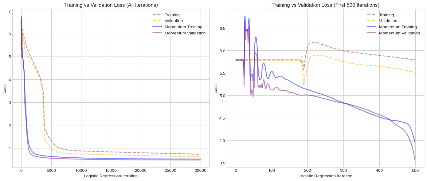
Momentum definitely had an effect on the convergence speed of the model! At around 1000 and definitely by 5000 iterations we see that the loss has essentially plateaued. On the other hand, our vanilla logistic regression that only really got there around 6000 and could keep training even after 30000 iterations. I found the first 500 iterations especially fascinating. We can see that our momentum may have sent us too far in the wrong direction at times, causing the loss to jump up before eventually steadying out and beginning to trend in the right direction. With respect to this issue, it would be interesting to implement variable learning rates throughout the process, possibly starting very small and as we begin to movement in the right direction we can increase the step size (similar to how momentum works) and do the inverse when we go in teh wrong direction. We could also think about variable momentum coefficients that work in a similar fashion. One interesting factor to observe is that our validation loss was consistently lower that our training loss which I honestly cannot explain for the moment apart from luck with the validation set. Nonetheless, we can observe that momentum was a significant optimizing factor in training our model.
In this post, we implemented a logistic regression model and conducted a series of experiments to better understand its behavior. We started off using a simple two-dimensional dataset to compare vanilla gradient descent with momentum aided descent. We demonstrated that momentum can smooth the convergence process and accelerate progress in a clean, linearly separable context. We then tackled the issue of overfitting by experimenting with scenarios where the number of features exceeded the number of data points, highlighting some of the pitfalls of excessive model complexity. Finally, we applied the model to predict World Cup match winners using real match data. With very small learning rates and high iteration numbers we were able to achieve decent accuracy and loss. In the real-world scenario we still observed the benefits of introducing momentum as our model converged a lot faster using momentum. In conclusion, these experiments deepened my understanding of model implementation and optimization, the balance required to prevent the dangers of overfitting, and challenges applying logistic regression to real-world applications. We also outlined some further optimizations concerning variable parameters that we could implement in the future.